The Encrypted Game of Life in Python Using Concrete

The Game of Life was invented in 1970 by John Horton Conway. This life simulation consists basically in a grid, of a chosen size, starting from a random value, and being updated with rules, at every iteration. Graphical representation of these grids shows impressing resemblances with living systems that evolve or structures that seem to move. 

Most of the developers reading this blog post have heard or implemented the Game of Life, at a moment, during their studies or personal coding experiments. It’s at the same time easy to explain and fascinating to look at.

At Zama, we have a longstanding history with the Game of Life. Of course, the Game of Life is not an actual use case for privacy-preserving computations or for our customers, who are more interested in implementing health diagnostics on encrypted personal data or making financial predictions over encrypted wallets. Nevertheless, thanks to the inherently enjoyable nature of this life simulation, two blog posts have been written about the Game of Life using Zama's libraries: the first titled “Concrete Boolean and Conway’s Game of Life: A Tutorial” by Optalysys, demonstrated how to code the game using a version of our library that is now deprecated; the second: “The Game of Life : Rebooted” authored by our colleagues at Zama, refined the implementation and achieved speed improvements in TFHE-rs. Both were primarily written in Rust.

In this new article, we explain how to code the Game of Life in Python using Zama library: Concrete. Writing this game in Python provides us with an enjoyable opportunity to demonstrate the typical process for a developer, especially how to make their program more efficient. We provide a link to and description of our ready-to-use implementation, which you can execute on your own machine.

The rules

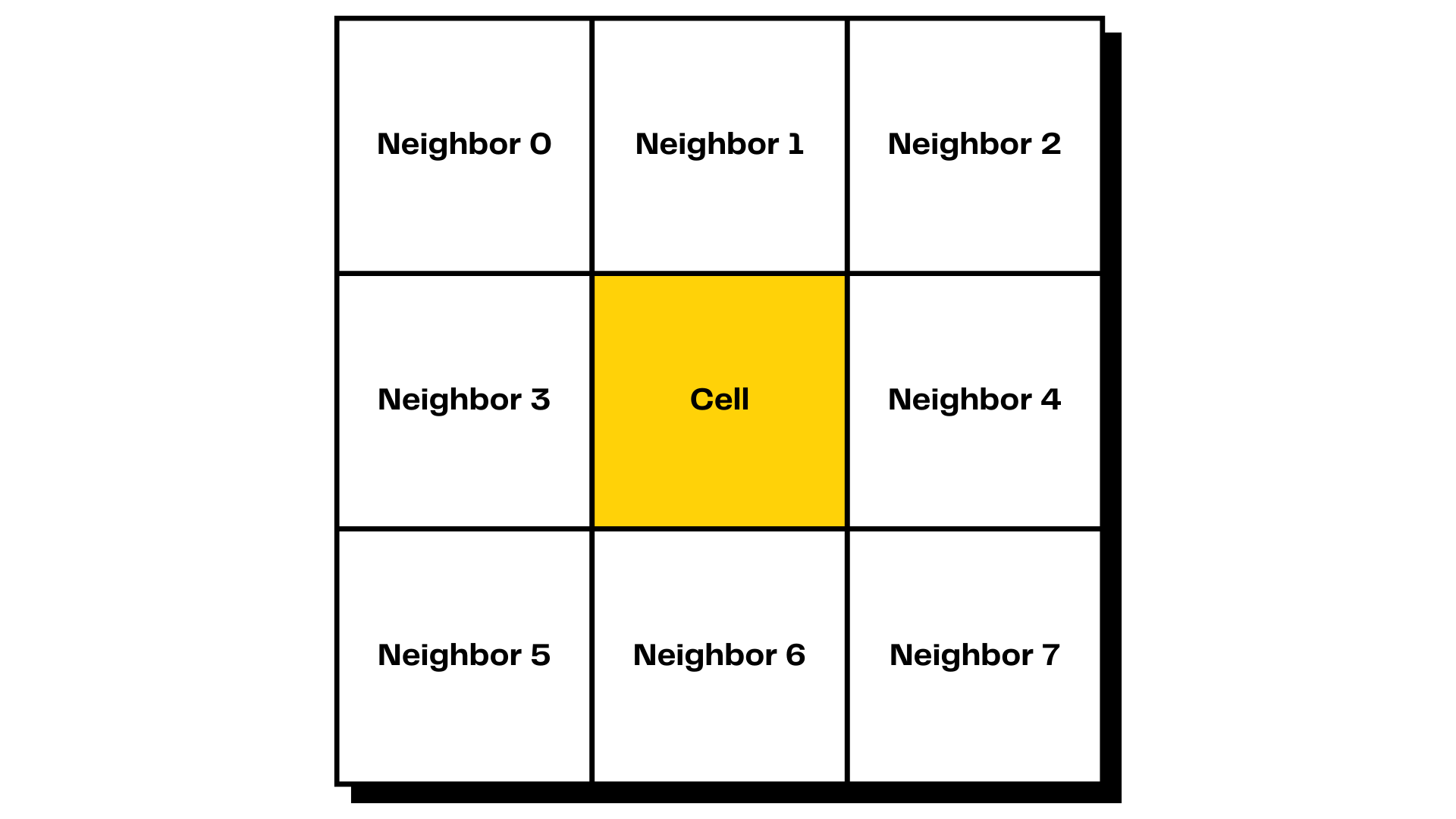
The rules of the Game of Life are quite straightforward: a grid represents the board, and cells are either active or inactive, or, let's say, alive or dead. At each iteration, the grid is updated according to the following principles. For each cell on the grid, we count the number of living neighbours (each cell has 8 neighbours, except for those on the edges of the grid):

• If the cell is active and has 2 or 3 active neighbours, the cell remains active; it survives.
• If the cell is inactive and has exactly 3 active neighbours, the cell becomes active; it is born.
• In all other cases, the cell becomes inactive; it dies.

We direct interested readers to the extensive literature on the Game of Life for studies about the various intriguing structures within it, such as those that move, replicate, or remain in equilibrium. Here, we will simply treat this function as an enjoyable game to implement and optimize using our libraries.

Coding The Game of Life in Python

One straightforward method to code the Game of Life in Python is to: (i) use a two-dimensional NumPy array for the grid, designating 1s for living cells and 0s for dead cells; (ii) count the number of active neighbors for a given cell at position (i, j); and (iii).

grid[i, j] = (nb_active_neighbors == 3) | (grid[i, j] & (nb_active_neighbors == 2))

Here, we can see the rules in action: a cell becomes or remains alive only if it has three neighbors, or if it is already alive and has two neighbors. To calculate the number of active neighbors, we could iterate over the adjacent cells, or we could use the convolution operator, which is commonly used in machine learning. We will employ the latter approach in our implementation.

Implementing in Concrete Python

Concrete Python enables the coding of various types of programs and provides a wide array of tensor operators, especially since it is utilized in the Concrete ML library. This library enhances classical machine learning frameworks such as scikit-learn, PyTorch, XGBoost, TensorFlow, or ONNX with privacy features.

In Concrete Python, there is a particularly useful operator for non-linear operations: the lookup table. Typically, we can apply a table of our choice to the grid. In our case, we will code the update process using this operator:

nb_active_neighbors = Conv(grid, W)
grid = T_a[nb_active_neighbors] | (grid & T_b[nb_active_neighbors])

where 

• W is the convolution matrix: W = np.array([[1, 1, 1], [1, 0, 1], [1, 1, 1]]).
• T_a and T_b are tables of 9 elements (since the input to the table, which is the number of active neighbors, stands between 0 and 8, included), with T_a[i] = 1 for i == 3 and 0 for other i’s, and T_b[i] = 1 for i in [2, 3] and 0 for other i’s.

As one can see, this implementation is quite easy to understand and naturally adheres to the rules of the game. However, in the subsequent paragraphs, we will see that it is possible to devise other implementations that are much more efficient.

Installing the code

Our code, along with all the implementations described in this blog post, is available in our repository. To demonstrate the process of writing more efficient code, let's explain how to install it. Essentially, one should follow these steps:

git clone https://github.com/zama-ai/concrete.git
cd docs/application-tutorial/
python3 -m venv .venv
source .venv/bin/activate
pip3 install -U pip wheel setuptools --ignore-installed
pip3 install -r game_of_life.requirements.txt --ignore-installed

Running a simulation or the FHE version

Once everything is installed, one can run the simulation (i.e., without actual encryption, for debugging purposes) or the real Fully Homomorphic Encryption (FHE) execution by choosing whether to use the [.c-inline-code]--simulate[.c-inline-code] flag. As expected, computations in simulations are much faster and can be utilized when testing new implementations of the grid update function. After ensuring everything works in simulations, one can proceed to execute in FHE. It is advisable to use powerful machines for FHE executions.

# In simulation
python3 game_of_life.py --dimension 100 --refresh_every 50 --simulate

# In FHE
python3 game_of_life.py --dimension 10 --refresh_every 10 

The basic implementation

To view our basic implementation (which corresponds to the [.c-inline-code]update_grid_basic[.c-inline-code] function in our code), one can use the [.c-inline-code]--show_mlir[.c-inline-code] and [.c-inline-code]--stop_after_compilation[.c-inline-code] options. Adding these flags enables one to see the MLIR (Multi-Level Intermediate Representation), which is the intermediate representation of the program used by the compiler. For more explanation about MLIR and insights into how our compiler operates under the hood, please refer to our blog: “Concrete — Zama's Fully Homomorphic Encryption Compiler”.

python3 docs/application-tutorial/game_of_life.py --dimension 6 --refresh_every 8 --method method_basic --show_mlir --stop_after_compilation 

And here is the Multi-Level Intermediate Representation:

module {
  func.func @main(%arg0: tensor<1x1x6x6x!FHE.eint<4>>) -> tensor<1x1x6x6x!FHE.eint<1>> {
    %cst = arith.constant dense<[[[[1, 1, 1], [1, 0, 1], [1, 1, 1]]]]> : tensor<1x1x3x3xi5>
    %0 = "FHELinalg.conv2d"(%arg0, %cst) {dilations = dense<1> : tensor<2xi64>, group = 1 : i64, padding = dense<0> : tensor<4xi64>, strides = dense<1> : tensor<2xi64>} : (tensor<1x1x6x6x!FHE.eint<4>>, tensor<1x1x3x3xi5>) -> tensor<1x1x4x4x!FHE.eint<4>>
    %1 = "FHE.zero_tensor"() : () -> tensor<1x1x6x6x!FHE.eint<4>>
    %inserted_slice = tensor.insert_slice %0 into %1[0, 0, 1, 1] [1, 1, 4, 4] [1, 1, 1, 1] : tensor<1x1x4x4x!FHE.eint<4>> into tensor<1x1x6x6x!FHE.eint<4>>
    %cst_0 = arith.constant dense<[0, 0, 0, 1, 0, 0, 0, 0, 0, 0, 0, 0, 0, 0, 0, 0]> : tensor<16xi64>
    %2 = "FHELinalg.apply_lookup_table"(%inserted_slice, %cst_0) : (tensor<1x1x6x6x!FHE.eint<4>>, tensor<16xi64>) -> tensor<1x1x6x6x!FHE.eint<1>>
    %cst_1 = arith.constant dense<[0, 0, 1, 1, 0, 0, 0, 0, 0, 0, 0, 0, 0, 0, 0, 0]> : tensor<16xi64>
		%3 = "FHELinalg.apply_lookup_table"(%inserted_slice, %cst_1) : (tensor<1x1x6x6x!FHE.eint<4>>, tensor<16xi64>) -> tensor<1x1x6x6x!FHE.eint<1>>
    %c1_i2 = arith.constant 1 : i2
    %cst_2 = arith.constant dense<[0, 1, 0, 0, 0, 0, 0, 0, 0, 0, 0, 0, 0, 0, 0, 0]> : tensor<16xi64>
    %4 = "FHELinalg.apply_lookup_table"(%arg0, %cst_2) : (tensor<1x1x6x6x!FHE.eint<4>>, tensor<16xi64>) -> tensor<1x1x6x6x!FHE.eint<1>>
    %cst_3 = arith.constant dense<[0, 2]> : tensor<2xi64>
    %5 = "FHELinalg.apply_lookup_table"(%3, %cst_3) : (tensor<1x1x6x6x!FHE.eint<1>>, tensor<2xi64>) -> tensor<1x1x6x6x!FHE.eint<2>>
    %cst_4 = arith.constant dense<[0, 1]> : tensor<2xi64>
    %6 = "FHELinalg.apply_lookup_table"(%4, %cst_4) : (tensor<1x1x6x6x!FHE.eint<1>>, tensor<2xi64>) -> tensor<1x1x6x6x!FHE.eint<2>>
    %7 = "FHELinalg.add_eint"(%5, %6) : (tensor<1x1x6x6x!FHE.eint<2>>, tensor<1x1x6x6x!FHE.eint<2>>) -> tensor<1x1x6x6x!FHE.eint<2>>
    %cst_5 = arith.constant dense<[0, 0, 0, 1]> : tensor<4xi64>
    %8 = "FHELinalg.apply_lookup_table"(%7, %cst_5) : (tensor<1x1x6x6x!FHE.eint<2>>, tensor<4xi64>) -> tensor<1x1x6x6x!FHE.eint<1>>
    %9 = "FHELinalg.apply_lookup_table"(%2, %cst_3) : (tensor<1x1x6x6x!FHE.eint<1>>, tensor<2xi64>) -> tensor<1x1x6x6x!FHE.eint<2>>
    %10 = "FHELinalg.apply_lookup_table"(%8, %cst_4) : (tensor<1x1x6x6x!FHE.eint<1>>, tensor<2xi64>) -> tensor<1x1x6x6x!FHE.eint<2>>
    %11 = "FHELinalg.add_eint"(%9, %10) : (tensor<1x1x6x6x!FHE.eint<2>>, tensor<1x1x6x6x!FHE.eint<2>>) -> tensor<1x1x6x6x!FHE.eint<2>>
    %cst_6 = arith.constant dense<[0, 1, 1, 1]> : tensor<4xi64>
    %12 = "FHELinalg.apply_lookup_table"(%11, %cst_6) : (tensor<1x1x6x6x!FHE.eint<2>>, tensor<4xi64>) -> tensor<1x1x6x6x!FHE.eint<1>>
    return %12 : tensor<1x1x6x6x!FHE.eint<1>>
  }
}

As one can observe, the MLIR is quite complex because this code was not optimized for speed in FHE. In particular, there are several table lookups, which you can identify as [.c-inline-code]apply_lookup_table[.c-inline-code]. These operations, known as PBS (Programmable Bootstrapping) in the FHE realm, are among the slowest in FHE. Therefore, it is in the developer's interest to:

• Try to limit the number of PBS operations.
• Reduce the size of their inputs, i.e., use smaller lookup tables.

In the [.c-inline-code]update_grid_basic[.c-inline-code] function, there are three PBS operations of 4 bits, two PBS operations of 3 bits, and four PBS operations of 2 bits. As indicated in the final table with execution timings, this is not the fastest implementation possible. In the following sections, we will explain how we have implemented other updates and measure them on an m6i machine to determine the most efficient one in practice.

Speeding up our implementation

5 bit PBS method. Our first idea was the one described in function [.c-inline-code]update_grid_method_5b[.c-inline-code]. Here, we use a slightly different convolution matrix: [.c-inline-code]W = np.array([[1, 1, 1], [1, 9, 1], [1, 1, 1]])[.c-inline-code]. Then, we apply a single table look up 18-byte-long [.c-inline-code]T_5b[.c-inline-code], which is 0 everywhere, but for indices 3, 9 + 2 and 9 + 3 where the table value is 1. Why?, you would ask. 

Indeed:

Which explains why we have chosen this value for the [.c-inline-code]T_5b[.c-inline-code] table.

python3 docs/application-tutorial/game_of_life.py --dimension 6 --refresh_every 8 --method method_5b --show_mlir --stop_after_compilation

You then see that the MLIR code is much simpler:

module {
  func.func @main(%arg0: tensor<1x1x6x6x!FHE.eint<5>>) -> tensor<1x1x6x6x!FHE.eint<1>> {
    %cst = arith.constant dense<[[[[1, 1, 1], [1, 9, 1], [1, 1, 1]]]]> : tensor<1x1x3x3xi6>
    %0 = "FHELinalg.conv2d"(%arg0, %cst) {dilations = dense<1> : tensor<2xi64>, group = 1 : i64, padding = dense<0> : tensor<4xi64>, strides = dense<1> : tensor<2xi64>} : (tensor<1x1x6x6x!FHE.eint<5>>, tensor<1x1x3x3xi6>) -> tensor<1x1x4x4x!FHE.eint<5>>
    %1 = "FHE.zero_tensor"() : () -> tensor<1x1x6x6x!FHE.eint<5>>
    %inserted_slice = tensor.insert_slice %0 into %1[0, 0, 1, 1] [1, 1, 4, 4] [1, 1, 1, 1] : tensor<1x1x4x4x!FHE.eint<5>> into tensor<1x1x6x6x!FHE.eint<5>>
    %cst_0 = arith.constant dense<[0, 0, 0, 1, 0, 0, 0, 0, 0, 0, 0, 1, 1, 0, 0, 0, 0, 0, 0, 0, 0, 0, 0, 0, 0, 0, 0, 0, 0, 0, 0, 0]> : tensor<32xi64>
    %2 = "FHELinalg.apply_lookup_table"(%inserted_slice, %cst_0) : (tensor<1x1x6x6x!FHE.eint<5>>, tensor<32xi64>) -> tensor<1x1x6x6x!FHE.eint<1>>
    return %2 : tensor<1x1x6x6x!FHE.eint<1>>
  }
}

Here, we have a single PBS, but it’s a 5 bit PBS, since the output of the convolution of W is between 0 and 17. 

4 bit PBS method. Our second idea was the one described in function [.c-inline-code]update_grid_method_4b[.c-inline-code]. We come back to the convolution matrix: [.c-inline-code]W = np.array([[1, 1, 1], [1, 0, 1], [1, 1, 1]])[.c-inline-code]. Then, we apply a first table [.c-inline-code]T_4b_a[.c-inline-code], add the grid to the result of the convolution, and apply a second table [.c-inline-code]T_4b_b[.c-inline-code]. We have defined [.c-inline-code]T_4b_a[.c-inline-code] as [.c-inline-code][i - 1 if i in [2, 3] else 0 for i in range(9)][.c-inline-code], and [.c-inline-code]T_4b_b[.c-inline-code] as [.c-inline-code][i in [2, 3] for i in range(4)][.c-inline-code]. 

The idea is the following:

• If the number of neighbours is 2: the output of [.c-inline-code]T_4b_a[.c-inline-code] will be 1.
• If the number of neighbours is 3: the output of [.c-inline-code]T_4b_a[.c-inline-code] will be 2.
• Else, [.c-inline-code]T_4b_a[.c-inline-code] will be 0.

Such that, after the addition with the grid, we get

• If the number of neighbours is 2: the input to[.c-inline-code] T_4b_b[.c-inline-code] will be 1 + cell.
• If the number of neighbours is 3: the input to [.c-inline-code]T_4b_b[.c-inline-code] will be 2 + cell.
• Else, input of [.c-inline-code]T_4b_b[.c-inline-code] will be cell.

And, looking at the definition of [.c-inline-code]T_4b_b[.c-inline-code], we have that the final result is 1 if and only if:

• the number of neighbours is 2 and cell is active.
• or, the number of neighbours is 3.

Which is exactly the rules of Game of Life.

The command:

python3 docs/application-tutorial/game_of_life.py --dimension 6 
--refresh_every 8 --method method_4b --show_mlir 
--stop_after_compilation

The MLIR corresponding to the new implementation will be displayed. In this version, we have two PBS operations: one with 4 bits and one with 2 bits. This may be faster than the previous 5-bit implementation, depending on the target machine.

3-bit PBS method. Our third approach is described in the function [.c-inline-code]update_grid_method_3b[.c-inline-code]. We leave it as an exercise for the reader to understand the method and will simply note here that this method results in three PBS operations: two with 3 bits and one with 2 bits.

Running the code over a m6i machine

To assess the efficiency of the different methods in practice, we executed our code in FHE on an m6i machine, using 200*200 grids with Concrete Python 2.4, and set the probability of error to 2^-40.  The typical command line for this operation is: [.c-inline-code]python3 game_of_life.py --dimension 200 --refresh_every 10 --log2_p_error -40 --method method_3b[.c-inline-code] We also executed the code on 6*6 grids, but since execution times are shorter for smaller grids, the differences between the implementations are less pronounced.

Algorithmically, the execution time increases with the square of the grid dimension. However, there are also some constant overheads to consider. It is also noteworthy that increasing the probability of error can significantly speed up computations.

Our 6*6 grid timings are notably faster than those previously reported in the Optalysys blog post (about one minute per update on an Intel i7 @ 3.6 GHz) and in the earlier Zama blog post (about 4.5 seconds on an Intel Core i5 @ 2.7 GHz). For a fair comparison, it should be mentioned that our implementation is multi-threaded (which is automatically managed by our compiler), unlike those in the aforementioned blogs, and it was executed on a more powerful m6i machine.

For a complete state of the art, let's also acknowledge the implementation by KU Leuven: in their presentation at the FHE.org 2023 conference, they demonstrated that FPGA implementations (as opposed to pure CPU implementations) can achieve about 60 ms for a 6*6 grid.

Conclusion

In this blog post, we conducted experiments with Concrete to explore how to implement a function (in this case, the Game of Life) with significantly faster execution times. Accelerating implementations is particularly crucial for the various machine learning algorithms that we have incorporated into our library and remains a constant goal for us at different levels: cryptography, compiler, and library. As we have demonstrated, users can also impact performance by understanding how their algorithms work in FHE and by optimizing to minimize speed impact.

Additional links

• Star the Concrete Github repository to endorse our work.
• Review the Concrete documentation.
• Get support on our community channels.
• Help advance the FHE space with the Zama Bounty Program.